一、DINO 是什么? 在视觉表征学习方向,无需人工标注的自监督学习方法逐渐成为主流,但是以往的方法几乎都依赖大量负样本来维持训练稳定,但负样本选择与内存消耗始终是一个瓶颈。
2021年,DINO(Self-Distillation with No Labels)横空出世,它仅通过教师–学生自蒸馏框架 与多视角数据增强 ,在没有负样本的情况下也能学到极具语义的特征表示。更令人惊讶的是,当DINO应用于ViT时,注意力图自发地对齐了图像中的物体区域,展现出强大的“涌现性质”,使其成为自监督视觉表征学习发展中的重要里程碑。
二、DINO的核心原理 2.1 多视角数据增强 对于一张图片,将其做2次全局数据增强以及N次局部数据增强。全局增强意味着该增强视图可以表征输入图片的全局信息,通常是224x224大小;而局部增强的视图尺寸通常只有96x96,仅覆盖了输入图片的局部信息。
2张全局增强的视图被作为教师网络的输入,2张全局增强+N次局部增强的视图被作为学生网络的输入。
在训练时,学生网络不仅要学会与教师网络全局视角的对齐,还要学习如何将局部视角与教师网络的全局视角进行对齐,从而激发学生网络的“涌现能力”。
上述数据增强的代码如下:
1
2
3
4
5
6
7
8
9
10
11
12
13
14
15
16
17
18
19
20
21
22
23
24
25
26
27
28
29
30
31
32
33
34
35
36
37
38
39
40
41
42
43
44
45
46
class DataAugmentationDINO (object ): def __init__ (self, global_crops_scale, local_crops_scale, local_crops_number ): flip_and_color_jitter = transforms.Compose([ transforms.RandomHorizontalFlip(p=0.5 ), transforms.RandomApply( [transforms.ColorJitter(brightness=0.4 , contrast=0.4 , saturation=0.2 , hue=0.1 )], p=0.8 ), transforms.RandomGrayscale(p=0.2 ), ]) normalize = transforms.Compose([ transforms.ToTensor(), transforms.Normalize((0.485 , 0.456 , 0.406 ), (0.229 , 0.224 , 0.225 )), ]) self .global_transfo1 = transforms.Compose([ transforms.RandomResizedCrop(224 , scale=global_crops_scale, interpolation=Image.BICUBIC), flip_and_color_jitter, utils.GaussianBlur(1.0 ), normalize, ]) self .global_transfo2 = transforms.Compose([ transforms.RandomResizedCrop(224 , scale=global_crops_scale, interpolation=Image.BICUBIC), flip_and_color_jitter, utils.GaussianBlur(0.1 ), utils.Solarization(0.2 ), normalize, ]) self .local_crops_number = local_crops_number self .local_transfo = transforms.Compose([ transforms.RandomResizedCrop(96 , scale=local_crops_scale, interpolation=Image.BICUBIC), flip_and_color_jitter, utils.GaussianBlur(p=0.5 ), normalize, ]) def __call__ (self, image ): crops = [] crops.append(self .global_transfo1(image)) crops.append(self .global_transfo2(image)) for _ in range (self .local_crops_number): crops.append(self .local_transfo(image)) return crops
使用dataset = datasets.ImageFolder(args.data_path, transform=transform)来定义DataSet类,其中的transform = DataAugmentationDINO(…),然后用DataLoader类进行包裹得到数据加载器。
对于数据加载器中的每一次迭代,都可以取到一个列表crops,里面包含多个增强视图,其中前两个元素是全局视图,后面的均为局部视图。比如,假设batch_size=64,局部视图数量N=8,那么一次迭代拿到的内容为:
1
2
3
4
5
6
7
crops = [ tensor([64, 3, 224, 224]), # global crop 1 tensor([64, 3, 224, 224]), # global crop 2 tensor([64, 3, 96, 96]), # local crop 1 ... tensor([64, 3, 96, 96]) # local crop 8 ]
由于存在两种不同的尺寸,为了加速处理,官方代码定义了一个MultiCropWrapper类,它的原理如下:
首先,将上面的crops列表按照尺寸进行分组:
1
2
3
4
idx_crops = torch.cumsum(torch.unique_consecutive( torch.tensor([inp.shape[-1 ] for inp in crops]), return_counts=True )[1 ], 0 )
这里crops[-1]的H或W可以区分不同crop,得到idx_crops=[2, 10].
分组之后,分批送入基于ViT架构的backbone
1 2 3 4 5 6 7 _out_global = backbone(torch.cat(images[0 :2 ])) _out_local = backbone(torch.cat(images[2 :10 ]))
这里之所以可以统一不同尺寸的维度到embed_dim,是因为最终只取了ViT输出序列维度的CLS token这一维([1,embed_dim]),其中存储了所有patch融合后的信息。
最后,将不同尺寸的特征进行拼接后,送入最终的head即可:
1
2
3
4
output = torch.cat([_out_global, _out_local]) # shape -> [128 + 512, embed_dim] = [640, embed_dim] final_output = head(output) # shape -> [640, out_dim]
其中,
1
2
3
4
5
6
7
8
9
10
final_output[0:64] → 全局crop1, 样本 0~63 final_output[64:128] → 全局crop2, 样本 0~63 final_output[128:192] → 局部crop1, 样本 0~63 … final_output[576:640] → 局部crop8, 样本 0~63
注意,在后续计算loss时,直接使用上述[640, out_dim]的final_output即可,无需再次将shape变换回去。
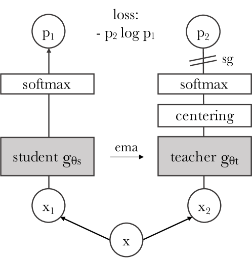
2.2 教师-学生自蒸馏框架 DINO采用了一种教师–学生自蒸馏框架,两个模型的网络架构是一模一样的,均基于ViT。
只不过,教师网络的梯度追踪是关闭状态,它的参数在训练之前被初始化为与学生网络一样的参数,后续通过学生网络的EMA进行参数更新,而非反向传播:
对应的代码实现为:
1
2
3
4
with torch.no_grad(): m = momentum_schedule[it] for param_s, param_t in zip (student.module.parameters(), teacher_without_ddp.parameters()): param_t.data.mul_(m).add_((1 - m) * param_s.detach().data)
这里的动量m不是固定的,而是随着训练逐渐增大,一般使用余弦调度,这样可以初期让教师快速跟上学生,后期保持教师稳定,提高表示质量。
学生网络上正常执行反向传播的,target是教师网络的输出,使用交叉熵作为损失函数。
在一次前向传播过程中,学生网络的输入和教师网络的输入是同一张图片的不同增强视图,教师网络只输入2个全局视图,学生网络输入2张全局视图+N张局部视图。
1
2
3
4
with torch.cuda.amp.autocast(fp16_scaler is not None ): teacher_output = teacher(images[:2 ]) student_output = student(images) loss = dino_loss(student_output, teacher_output, epoch)
三、DINO是如何在没有负样本的情况下避免模型崩塌的? 在训练时,模型的目标时让学生网络的输出尽可能和教师网络的输出接近。
然而,考虑一个极端情况,就是学生网络和教师网络都学会了偷懒:无论输入的图像增强视图是什么,两者都输出一个相同的常量,这样做无需继续学习就可以达到loss=0的理想状态。但是,模型参数根本无法被更新!这就是模型坍塌 。
为了应对模型坍塌,DINO采用的方式为:教师网络输出中心化+较低温度系数做锐化。
中心化处理可以让教师网络输出向量的每一个维度之间更加平滑稳定,而锐化则刚好相反,通过均衡两者,便可有效控制模型的坍塌。
此外,多视图增强和教师网络的EMA参数更新方式也在一定程度上抑制了模型坍塌:
多视图增强学生网络必须同时对齐教师网络的全局视图和局部视图,增加任务难度;
EMA使教师网络变化缓慢,提供稳定的训练目标,防止学生网络因目标不稳定而崩塌。
1 2 teacher_out = F.softmax((teacher_output - self .center) / temp, dim=-1 )
四、DINO的损失函数 DINO的loss定义如下:
1
2
3
4
5
6
7
8
9
10
11
12
13
14
15
16
17
18
19
20
21
22
23
24
25
26
27
28
29
30
31
32
33
34
35
36
37
38
39
40
41
42
43
44
45
46
47
48
49
50
51
52
53
54
55
56
57
58
59
60
61
62
63
64
65
66
67
68
69
70
71
72
73
74
75
class DINOLoss (nn.Module): def __init__ (self, out_dim, ncrops, warmup_teacher_temp, teacher_temp, warmup_teacher_temp_epochs, nepochs, student_temp=0.1 , center_momentum=0.9 ): super ().__init__() self .student_temp = student_temp self .center_momentum = center_momentum self .ncrops = ncrops self .register_buffer("center" , torch.zeros(1 , out_dim)) self .teacher_temp_schedule = np.concatenate(( np.linspace(warmup_teacher_temp, teacher_temp, warmup_teacher_temp_epochs), np.ones(nepochs - warmup_teacher_temp_epochs) * teacher_temp )) def forward (self, student_output, teacher_output, epoch ): """ 计算 DINO 损失: student_output: 学生网络输出,shape = [batch*ncrops, out_dim] teacher_output: 教师网络输出,shape = [2*batch, out_dim] (仅全局视图) """ student_out = student_output / self .student_temp student_out = student_out.chunk(self .ncrops) temp = self .teacher_temp_schedule[epoch] teacher_out = F.softmax((teacher_output - self .center) / temp, dim=-1 ) teacher_out = teacher_out.detach().chunk(2 ) total_loss = 0 n_loss_terms = 0 for iq, q in enumerate (teacher_out): for v in range (len (student_out)): if v == iq: continue loss = torch.sum (-q * F.log_softmax(student_out[v], dim=-1 ), dim=-1 ) total_loss += loss.mean() n_loss_terms += 1 total_loss /= n_loss_terms self .update_center(teacher_output) return total_loss @torch.no_grad() def update_center (self, teacher_output ): """ 使用 EMA 更新教师输出中心 center """ batch_center = torch.sum (teacher_output, dim=0 , keepdim=True ) dist.all_reduce(batch_center) batch_center = batch_center / (len (teacher_output) * dist.get_world_size()) self .center = self .center * self .center_momentum + batch_center * (1 - self .center_momentum)
可以看到,在计算loss前,对教师网络进行了中心化+温度缩放来避免模型坍塌,中心化参数center是通过EMA方式更新的。注意这里的EMA是对中心center的更新,只不过和教师网络权重更新方式一样都采用了EMA。
在计算loss时,学生网络的每一个增强视图都和教师网络的2个全局增强视图进行了loss计算,但会跳过与教师视图对应的同视图,从而避免同视图直接匹配。
假设学生网络有ncrops=2+N个视图(2个全局+N个局部),那么每个batch总共会计算2*(1+N)=2+2N次交叉熵损失,然后再取平均得到最终的DINOLoss。
1
2
3
4
5
6
7
8
9
10
11
12
13
2+2N的由来: 教师有2个视图,所以外层循环次数=2 学生有ncrops=2+N个视图 内层循环中,每次会跳过与教师同视图的索引 当iq=0时,跳过v=0 → 内层循环有效次数=(2+N)-1=1+N 当iq=1时,跳过v=1 → 内层循环有效次数=(2+N)-1=1+N 总计计算loss次数为2*(1+N)=2+2N
这样的设计保证了学生网络在学习全局信息的同时,也充分利用了局部视图进行对齐,从而增强了特征表示的鲁棒性和语义丰富性。
参考: