从零开始实现YOLOv1

一、核心思想

• 1. YOLOv1 的核心思想是将目标检测问题视为一个回归问题，是一个直接从图像像素到边界框坐标及类别的映射。
• 2. 输入图像通过一个单一的CNN进行处理，网络将图像划分为多个网格，每个网格负责检测图像中一个目标。
• 3. 每个网格输出一个固定数量(B)的边界框和类别概率分布。

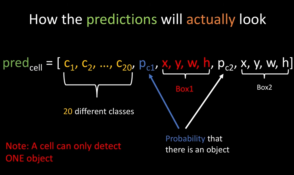
具体来说，Yolov1将一个448x448的原图片分割为7x7=49个网格(grid cell)，每个grid cell预测：

• B(论文中B=2)个边界框(bbox)的坐标(x,y,w,h)
• B个bbox内各自是否包含目标的置信度confidence
• 1个类别概率分布C

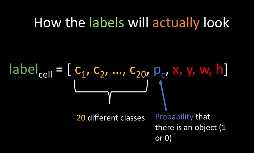
YOLOv1使用的训练集为pascal VOC2012，总共20个类别，因此每一个grid cell对应 (4+1)x2+20=30个预测参数。

二、标签格式

标签分为预测标签prediction和真实标签target.

target

首先明确，每个物体都有一个中心点，如下图蓝色点所示。

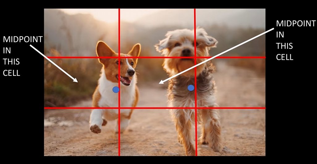
每个gird cell都只负责预测某物体中心点落入该grid cell的物体。

比如左侧狗子的中心点落入了第二行第一列的grid cell，将其单独取出来：

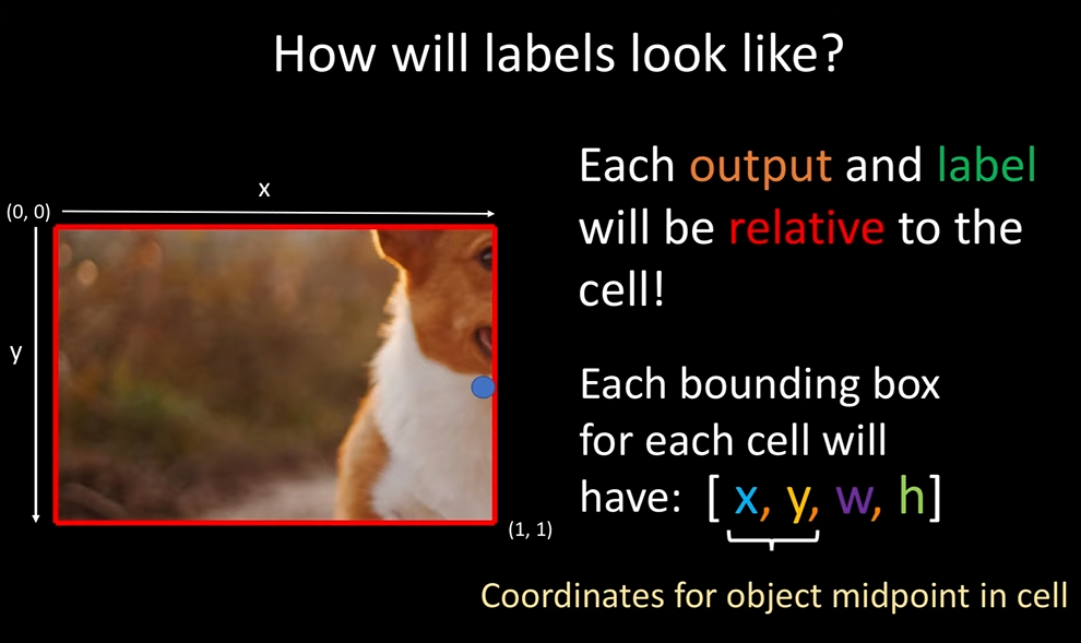
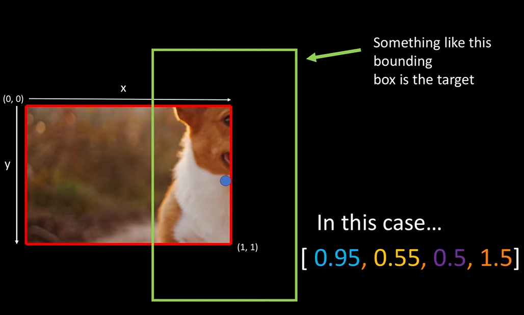
这里的 [x,y,w,h]是相对于该grid cell的左上角点(0,0)的，在上面的例子中，可能的值是[0.95,0.55,0.5,1.5]，如下图绿色框所示

因此，每个grid cell对应的target标签为：

prediction

预测标签prediction和target很像，只不过，prediction会预测2个bbox(以应对目标可能的两种比例：长>宽 or宽>长).

对比target和prediction

以上所介绍的均对于一个grid cell，而YOLOv1中将图像划分成了SxS个grid cell，因此，对于一张图片来说：

• target的shape：[S,S,4+1+20=25]
• prediction的shape：[S,S,2*(4+1)+20=30]

三、网络结构

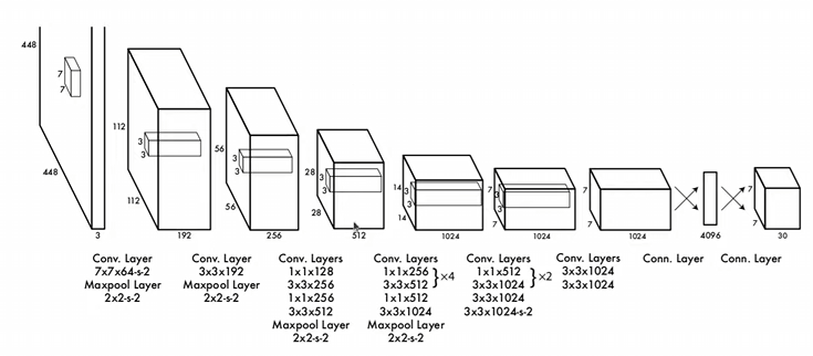
YOLOv1的网络结构很简单，直接上代码：

import torch
import torch.nn as nn

""" 
Information about architecture config:
Tuple is structured by (kernel_size, filters, stride, padding) 
"M" is simply maxpooling with stride 2x2 and kernel 2x2
List is structured by tuples and lastly int with number of repeats
"""

architecture_config = [
    # Tuple: (kernal_size,out_channels,stride,padding)
    (7, 64, 2, 3),
    "M",
    (3, 192, 1, 1),
    "M",
    (1, 128, 1, 0),
    (3, 256, 1, 1),
    (1, 256, 1, 0),
    (3, 512, 1, 1),
    "M",
    # Tuple: (kernal_size,out_channels,stride,padding) and number of repeats
    [(1, 256, 1, 0), (3, 512, 1, 1), 4],
    (1, 512, 1, 0),
    (3, 1024, 1, 1),
    "M",
    [(1, 512, 1, 0), (3, 1024, 1, 1), 2],
    (3, 1024, 1, 1),
    (3, 1024, 2, 1),
    (3, 1024, 1, 1),
    (3, 1024, 1, 1),
]


class CNNBlock(nn.Module):
    def __init__(self, in_channels, out_channels, **kwargs):
        super(CNNBlock, self).__init__()
        self.conv = nn.Conv2d(in_channels, out_channels, bias=False, **kwargs)
        self.batchnorm = nn.BatchNorm2d(out_channels)
        self.leakyrelu = nn.LeakyReLU(0.1)

    def forward(self, x):
        return self.leakyrelu(self.batchnorm(self.conv(x)))


class Yolov1(nn.Module):
    def __init__(self, in_channels=3, **kwargs):
        super(Yolov1, self).__init__()
        self.architecture = architecture_config
        self.in_channels = in_channels
        self.darknet = self._create_conv_layers(self.architecture)
        self.fcs = self._create_fcs(**kwargs)

    def forward(self, x):
        x = self.darknet(x)
        print(x.shape) # torch.Size([2, 1024, 7, 7])
        return self.fcs(torch.flatten(x, start_dim=1))

    def _create_conv_layers(self, architecture):
        layers = []
        in_channels = self.in_channels

        for x in architecture:
            if type(x) == tuple:
                layers += [
                    CNNBlock(
                        in_channels, x[1], kernel_size=x[0], stride=x[2], padding=x[3],
                    )
                ]
                in_channels = x[1]

            elif type(x) == str:
                layers += [nn.MaxPool2d(kernel_size=(2, 2), stride=(2, 2))]

            elif type(x) == list:
                conv1 = x[0]
                conv2 = x[1]
                num_repeats = x[2]

                for _ in range(num_repeats):
                    layers += [
                        CNNBlock(
                            in_channels,
                            conv1[1],
                            kernel_size=conv1[0],
                            stride=conv1[2],
                            padding=conv1[3],
                        )
                    ]
                    layers += [
                        CNNBlock(
                            conv1[1],
                            conv2[1],
                            kernel_size=conv2[0],
                            stride=conv2[2],
                            padding=conv2[3],
                        )
                    ]
                    in_channels = conv2[1]

        return nn.Sequential(*layers)

    def _create_fcs(self, split_size, num_boxes, num_classes):
        S, B, C = split_size, num_boxes, num_classes

        # In original paper this should be
        # nn.Linear(1024*S*S, 4096),
        # nn.LeakyReLU(0.1),
        # nn.Linear(4096, S*S*(B*5+C))

        return nn.Sequential(
            nn.Flatten(),
            nn.Linear(1024 * S * S, 496),
            nn.Dropout(0.0),
            nn.LeakyReLU(0.1),
            # 总共SxS个cell，每个cell预测1个目标(类别数为C)，可能预测B个bbox，
            # 每个bbox有4个坐标信息+1个置信度信息
            nn.Linear(496, S * S * (C + B * 5)),
        )

if __name__ == '__main__':
    model = Yolov1(split_size=7,num_boxes=2, num_classes=20)
    print(model)
    x=torch.randn(2,3,448,448)# 原论文中使用的image size是448x448
    z=model(x)
    print(z.shape)# torch.Size([2, 1470]) ,1470 = 7x7*(20+2*5)

四、数据加载器

打开一个标签文件：

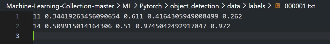
每一张图片对应一个.txt标注文件，标注文件中的每一行代表一个目标的信息(比如当前文件表明000001.png中包含两个目标)，从左到右分别是cls,x,y,w,h，并且是归一化的，这样即使图片做了resize，也不需要修改这些标注信息。

对于一张图片，模型预测结果的shape是[S,S,C+5xB]的，论文中B=2，且在划分正负样本后只有其中一个预测bbox与其对应的(如果有)的GT bbox计算loss，所以需要将上述标签文件中的信息转换成类似模型预测结果shape的格式。为此，首先搭建一个空的框架，其shape和模型预测结果shape保持一致：

label_matrix = torch.zeros((self.S, self.S, self.C + 5 * self.B))

(真实标签target只包含1个bbox，预测标签prediction包含B=2个bbox，这里的label_matrix虽然也包含B=2个bbox，但其中一个只是起到了占位的作用，只是为了方便编写代码)

接下来，基于每张图片中的若干个bbox的标注信息，针对每一条信息，定位该目标的中心点(x,y)在SxS的grid cell中对应的行和列，行和列唯一确定了一个grid cell，该grid cell负责预测该目标，并将这些信息填充到label_matrix对应的位置。处理完这张图片中的每一条信息后，就完成了label_matrix的填充。

但是，这些标注的位置信息是相对于整张图片的，而在计算loss时，需要的位置信息是相对于grid cell的左上角点的，因此在具体填充时，需要做进一步的转换操作。

具体来说，首先查看当前GT bbox属于哪个grid cell（GT bbox的中心点(x,y)落入的那个grid cell），然后将其转换到相对于所属grid cell的位置。

以下代码实现了上述文字所描述的功能：

# import torch
import os
import pandas as pd
from PIL import Image


class VOCDataset(torch.utils.data.Dataset):
    def __init__(
        self, csv_file, img_dir, label_dir, S=7, B=2, C=20, transform=None,
    ):
        self.annotations = pd.read_csv(csv_file)
        self.img_dir = img_dir
        self.label_dir = label_dir
        self.transform = transform
        self.S = S
        self.B = B
        self.C = C

    def __len__(self):
        return len(self.annotations)

    def __getitem__(self, index):
        # 处理标注
        label_path = os.path.join(self.label_dir, self.annotations.iloc[index, 1])
        boxes = []
        with open(label_path) as f:
            # 解析标注文件中的每一个目标
            for label in f.readlines():
                class_label, x, y, width, height = [
                    float(x) if float(x) != int(float(x)) else int(x)
                    for x in label.replace("\n", "").split()
                ]

                boxes.append([class_label, x, y, width, height])

        # 处理图片
        img_path = os.path.join(self.img_dir, self.annotations.iloc[index, 0])
        image = Image.open(img_path)
        boxes = torch.tensor(boxes)

        if self.transform:
            # image = self.transform(image)
            image, boxes = self.transform(image, boxes)

        # Convert To Cells
        # 将位置信息转换为相对于cell的
        label_matrix = torch.zeros((self.S, self.S, self.C + 5 * self.B))
        for box in boxes:
            class_label, x, y, width, height = box.tolist()
            class_label = int(class_label)

            # i,j represents the cell row and cell column # 定位到所属grid cell的（行，列）位置
            # x和y是归一化的，并且原始图片被划分为S*S个grid cell
            # 因此S * y和S * x 分别代表当前GT box所属的grid cell所在的行和列，也就定位到了当前GT box所属于的grid cell
            i, j = int(self.S * y), int(self.S * x) 

            # 接下来，开始执行xywh的转换
            # 首先是xy的转换：
            # 原来的中心点xy是相对于原始图片的，现在已知其所属grid cell的左上角点，
            # 直接将xy减去grid cell的左上角点坐标，就得到了相对于所属grid cell的中心点xy
            x_cell, y_cell = self.S * x - j, self.S * y - i

            """
            Calculating the width and height of cell of bounding box,
            relative to the cell is done by the following, with
            width as the example:
  
            width_pixels = (width*self.image_width)
            cell_pixels = (self.image_width)
  
            Then to find the width relative to the cell is simply:
            width_pixels/cell_pixels, simplification leads to the
            formulas below.
            """
            # 接着是wh的转换，只需要将归一化的相对于原图的wh乘以划分grid cell的数量
            width_cell, height_cell = (
                width * self.S,
                height * self.S,
            )

            # If no object already found for specific cell i,j
            # Note: This means we restrict to ONE object
            # per cell!
            # 如果当前grid cell还没有找到其所负责预测的GT bbox，那么就将当前的GT bbox分配给它
            if label_matrix[i, j, 20] == 0:
                # Set that there exists an object
                label_matrix[i, j, 20] = 1

                # Box coordinates
                box_coordinates = torch.tensor(
                    [x_cell, y_cell, width_cell, height_cell]
                )

                label_matrix[i, j, 21:25] = box_coordinates# 只是用第一个bbox的位置。另一个仅占位。

                # Set one hot encoding for class_label
                label_matrix[i, j, class_label] = 1

        return image, label_matrix

这里再次总结一下YOLOv1的思路：

将图片划分为SxS个grid cell，每个grid cell负责预测B个bbox来对应GT bbox(如果有对应的GT bbox与之匹配，且一对一，B=1个正样本+1个负样本；若无GT 匹配，B=2个负样本)。这里的“负责”指的是将该网格对应的预测bbox与其匹配的GT bbox之间求loss，不断地使得该网格负责预测的bbox接近与之匹配的GT bbox。“负责”的概念，其实只是逻辑上的，具体表现在人为构建的label_matrix的shape：(self.S, self.S, self.C + 5 x self.B)，正是因为人为从逻辑上将原图划分成了Sx*S个网格，才产生了“负责”的概念。模型预测SxS个grid cell的信息，上述构建的label_matrix也包含了SxS个grid cell的信息，shape已经对齐了，这样就可以计算loss了。

五、损失函数

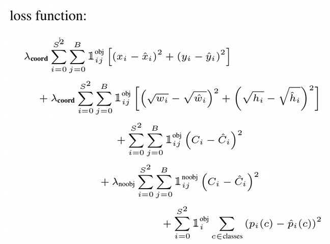
YOLOv1的所有损失函数均采用的MSE，其中：

• 第一行和第二行：bbox损失，第一行是中心点的损失计算，第二行是宽和高的损失计算
• 第三行：正样本的置信度损失计算
• 第四行：负样本的置信度损失计算
• 第五行：正样本的预测类别损失计算

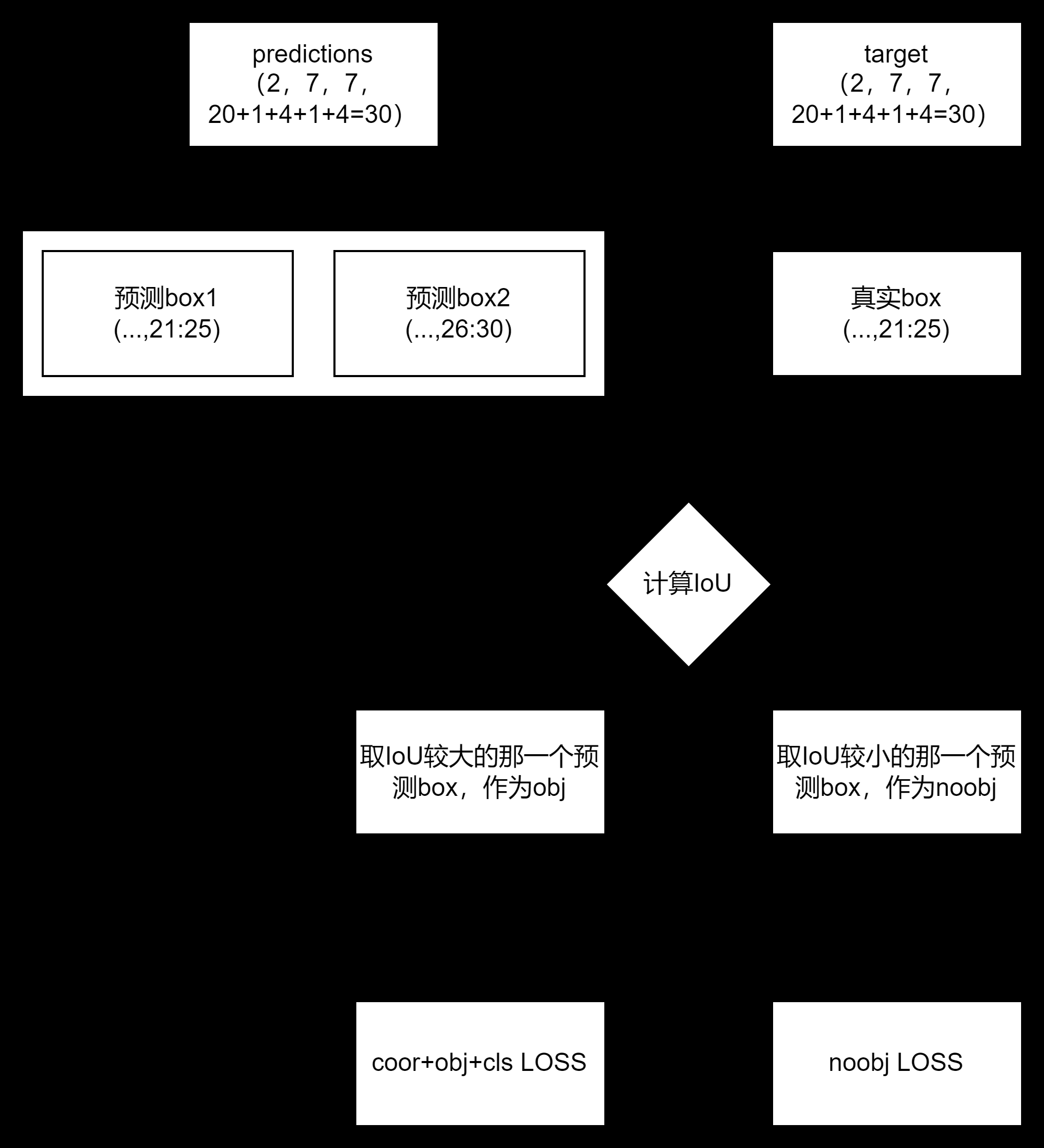
YOLOv1中的正负样本匹配策略：

总共SxS个grid cell，每个grid cell会预测B(B=2)个bbox，与GT bbox的IoU最大的预测bbox与GT bbox匹配，作为正样本参与loss计算（对应第一行、第二行和第三行）。

剩下的那个预测bbox作为负样本，只参与第四行的负样本置信度损失计算。

由于YOLOv1中每个grid cell只负责一个bbox，即使每个grid cell对应了B(B=2)个预测bbox，但是只有IoU最大的那个预测bbox才是正样本(有对应的GT bbox)，因此在第五行中，只有那些正样本参与类别损失计算。

上述逻辑的代码实现如下, 一些关键细节见代码注释：

import torch
import torch.nn as nn
from utils import intersection_over_union

class YoloLoss(nn.Module):
    """
    Calculate the loss for yolo (v1) model
    """

    def __init__(self, S=7, B=2, C=20):
        super(YoloLoss, self).__init__()
        self.mse = nn.MSELoss(reduction="sum")

        """
        S is split size of image (in paper 7),
        B is number of boxes (in paper 2),
        C is number of classes (in paper and VOC dataset is 20),
        """
        self.S = S
        self.B = B
        self.C = C

        # These are from Yolo paper, signifying how much we should
        # pay loss for no object (noobj) and the box coordinates (coord)
        self.lambda_noobj = 0.5
        self.lambda_coord = 5

    def forward(self, predictions, target):
        # predictions are shaped (BATCH_SIZE, S*S(C+B*5) when inputted, target as the same### [2, 7, 7, 30]
        predictions = predictions.reshape(-1, self.S, self.S, self.C + self.B * 5)# [2,7,7,30]

        # Calculate IoU for the two predicted bounding boxes with target bbox
        iou_b1 = intersection_over_union(predictions[..., 21:25], target[..., 21:25])# [2,7,7,1],2是batch_size
        iou_b2 = intersection_over_union(predictions[..., 26:30], target[..., 21:25])# [2,7,7,1]
        ious = torch.cat([iou_b1.unsqueeze(0), iou_b2.unsqueeze(0)], dim=0)# # [2,2,7,7,1] 第一个2是代表2个iou

        # Take the box with highest IoU out of the two prediction
        # Note that bestbox will be indices of 0, 1 for which bbox was best
        # iou_maxes：形状 [2, 7, 7, 1]，表示 每个网格在两个预测框中 IoU 最大的值。
        # bestbox：形状 [2, 7, 7, 1]，表示 IoU 最大的那个预测框的索引（0 或 1，因为B=2）。
        iou_maxes, bestbox = torch.max(ious, dim=0)# bestbox [2,7,7,1]
        exists_box = target[..., 20].unsqueeze(3)# [2,7,7,1]  # in paper this is Iobj_i

        # ======================== #
        #   FOR BOX COORDINATES    #
        # ======================== #

        # Set boxes with no object in them to 0. We only take out one of the two 
        # predictions, which is the one with highest Iou calculated previously.
        box_predictions = exists_box * (
            (   
                # 这里bestbox只取0或1，是作为正样本的预测box的索引下标，
                #如果bestbox是0，那么保留第0个预测box（xywh对应21:25），如果是1，保留第1个预测box（xywh对应26:30）
                bestbox * predictions[..., 26:30]
                + (1 - bestbox) * predictions[..., 21:25]
            )# best_box是0或者1，因此这里只会取与target的iou最大的预测box
        )# [2, 7, 7, 4]

        box_targets = exists_box * target[..., 21:25]# [2, 7, 7, 4]

        # Take sqrt of width, height of boxes to ensure that
        box_predictions[..., 2:4] = torch.sign(box_predictions[..., 2:4]) * torch.sqrt(
            torch.abs(box_predictions[..., 2:4] + 1e-6)
        )# 这里的一个小trick：abs确保数值为正，避免 sqrt 出现 NaN，sign获取原始值的正负号，以便保持原始符号，避免梯度爆炸或消失。
        box_targets[..., 2:4] = torch.sqrt(box_targets[..., 2:4])

        # 这里end_dim的作用：（BS,S,S, 4）flatten --> (BS*S*S, 4)
        box_loss = self.mse(
            torch.flatten(box_predictions, end_dim=-2),
            torch.flatten(box_targets, end_dim=-2),
        )

        # ==================== #
        #   FOR OBJECT LOSS    #
        # ==================== #

        # pred_box is the confidence score for the bbox with highest IoU
        pred_box = (
            bestbox * predictions[..., 25:26] + (1 - bestbox) * predictions[..., 20:21]
        )# pred_box这里预测的置信度得分！[2,7,7,1]

        # flatten -->（BS*S*S）
        object_loss = self.mse(
            torch.flatten(exists_box * pred_box),
            torch.flatten(exists_box * target[..., 20:21]),
        )

        # ======================= #
        #   FOR NO OBJECT LOSS    #
        # ======================= #

        #max_no_obj = torch.max(predictions[..., 20:21], predictions[..., 25:26])
        #no_object_loss = self.mse(
        #    torch.flatten((1 - exists_box) * max_no_obj, start_dim=1),
        #    torch.flatten((1 - exists_box) * target[..., 20:21], start_dim=1),
        #)
    
        # 如果不存在目标，那么预测的B(B=2)个bbox都是负样本，因此都需要参与noObj的置信度loss计算
        # 这里start_dim的作用：(BS,S,S,1) flatten --> (BS,S*S)，每一个预测bbox有1个置信度得分，
        # 因此这里是1，因为要分别计算两个预测bbox的noObj loss
        no_object_loss = self.mse(
            torch.flatten((1 - exists_box) * predictions[..., 20:21], start_dim=1),
            torch.flatten((1 - exists_box) * target[..., 20:21], start_dim=1),
        )

        no_object_loss += self.mse(
            torch.flatten((1 - exists_box) * predictions[..., 25:26], start_dim=1),
            torch.flatten((1 - exists_box) * target[..., 20:21], start_dim=1)
        )

        # ================== #
        #   FOR CLASS LOSS   #
        # ================== #
        # 这里end_dim的作用：(BS,S,S,20) flatten --> (BS*S*S,20)
        class_loss = self.mse(
            torch.flatten(exists_box * predictions[..., :20], end_dim=-2,),
            torch.flatten(exists_box * target[..., :20], end_dim=-2,),
        )


        # 可以看到，exists_box 充当了符号函数的作用，用于区分是否真的存在目标

        loss = (
            self.lambda_coord * box_loss  # first two rows in paper
            + object_loss  # third row in paper
            + self.lambda_noobj * no_object_loss  # forth row
            + class_loss  # fifth row
        )

        return loss

六、训练

训练代码就很常规的了，直接上代码：

"""
Main file for training Yolo model on Pascal VOC dataset

"""

import torch
import torchvision.transforms as transforms
import torch.optim as optim
import torchvision.transforms.functional as FT
from tqdm import tqdm
from torch.utils.data import DataLoader
from model import Yolov1
from dataset import VOCDataset
from utils import (
    non_max_suppression,
    mean_average_precision,
    intersection_over_union,
    cellboxes_to_boxes,
    get_bboxes,
    plot_image,
    save_checkpoint,
    load_checkpoint,
)
from loss import YoloLoss

seed = 123
torch.manual_seed(seed)

# Hyperparameters etc. 
LEARNING_RATE = 2e-5
DEVICE = "cuda" if torch.cuda.is_available else "cpu"
BATCH_SIZE = 16 # 64 in original paper but I don't have that much vram, grad accum?
WEIGHT_DECAY = 0
EPOCHS = 1000
NUM_WORKERS = 2
PIN_MEMORY = True
LOAD_MODEL = False
LOAD_MODEL_FILE = "overfit.pth.tar"
IMG_DIR = r"D:\MyFile\github\Machine-Learning-Collection-master\ML\Pytorch\object_detection\data\images"
LABEL_DIR = r"D:\MyFile\github\Machine-Learning-Collection-master\ML\Pytorch\object_detection\data\labels"


class Compose(object):
    def __init__(self, transforms):
        self.transforms = transforms

    def __call__(self, img, bboxes):
        for t in self.transforms:
            img, bboxes = t(img), bboxes

        return img, bboxes


transform = Compose([transforms.Resize((448, 448)), transforms.ToTensor(),])


def train_fn(train_loader, model, optimizer, loss_fn):
    loop = tqdm(train_loader, leave=True)
    mean_loss = []

    for batch_idx, (x, y) in enumerate(loop):
        x, y = x.to(DEVICE), y.to(DEVICE)
        out = model(x)
        loss = loss_fn(out, y)
        mean_loss.append(loss.item())
        optimizer.zero_grad()
        loss.backward()
        optimizer.step()

        # update progress bar
        loop.set_postfix(loss=loss.item())

    print(f"Mean loss was {sum(mean_loss)/len(mean_loss)}")


def main():
    model = Yolov1(split_size=7, num_boxes=2, num_classes=20).to(DEVICE)
    optimizer = optim.Adam(
        model.parameters(), lr=LEARNING_RATE, weight_decay=WEIGHT_DECAY
    )
    loss_fn = YoloLoss()

    if LOAD_MODEL:
        load_checkpoint(torch.load(LOAD_MODEL_FILE), model, optimizer)

    train_dataset = VOCDataset(
        r"D:\MyFile\github\Machine-Learning-Collection-master\ML\Pytorch\object_detection\data\100examples.csv",
        transform=transform,
        img_dir=IMG_DIR,
        label_dir=LABEL_DIR,
    )

    test_dataset = VOCDataset(
        r"D:\MyFile\github\Machine-Learning-Collection-master\ML\Pytorch\object_detection\data\test.csv", transform=transform, img_dir=IMG_DIR, label_dir=LABEL_DIR,
    )

    train_loader = DataLoader(
        dataset=train_dataset,
        batch_size=BATCH_SIZE,
        num_workers=NUM_WORKERS,
        pin_memory=PIN_MEMORY,
        shuffle=True,
        drop_last=True,
    )

    test_loader = DataLoader(
        dataset=test_dataset,
        batch_size=BATCH_SIZE,
        num_workers=NUM_WORKERS,
        pin_memory=PIN_MEMORY,
        shuffle=True,
        drop_last=True,
    )

    for epoch in range(EPOCHS):
        # for x, y in train_loader:
        #    x = x.to(DEVICE)
        #    for idx in range(8):
        #        bboxes = cellboxes_to_boxes(model(x))
        #        bboxes = non_max_suppression(bboxes[idx], iou_threshold=0.5, threshold=0.4, box_format="midpoint")
        #        plot_image(x[idx].permute(1,2,0).to("cpu"), bboxes)

        #    import sys
        #    sys.exit()

        pred_boxes, target_boxes = get_bboxes(
            train_loader, model, iou_threshold=0.5, threshold=0.4
        )

        mean_avg_prec = mean_average_precision(
            pred_boxes, target_boxes, iou_threshold=0.5, box_format="midpoint"
        )
        print(f"Train mAP: {mean_avg_prec}")

        #if mean_avg_prec > 0.9:
        #    checkpoint = {
        #        "state_dict": model.state_dict(),
        #        "optimizer": optimizer.state_dict(),
        #    }
        #    save_checkpoint(checkpoint, filename=LOAD_MODEL_FILE)
        #    import time
        #    time.sleep(10)

        train_fn(train_loader, model, optimizer, loss_fn)


if __name__ == "__main__":
    main()

以上就是本文关于YOLOv1的介绍，下一篇将介绍YOLOv3.